PyVBMC Example 7: Stacking the posteriors of several runs (S-VBMC)

In this notebook, we combine the variational posteriors of several independent PyVBMC runs into a single stacked posterior with S-VBMC (Stacking Variational Bayesian Monte Carlo; Silvestrin, Li & Acerbi, 2025).

Running PyVBMC several times from different starting points is standard practice to check that the runs agree (see Example 4). When they do not, for instance because the posterior is multimodal and each run captures only some of the modes, S-VBMC pools the mixture components of all runs and optimizes their weights against the stacked ELBO, using the expected log-joint statistics that every run already stores. Stacking therefore needs no further evaluations of the model.

This notebook is Part 7 of a series of notebooks in which we present various example usages for VBMC with the PyVBMC package. The code used in this example is available as a script here. S-VBMC needs the optional torch dependency: install it with pip install --upgrade "pyvbmc[torch]" (see the installation instructions for a CPU-only torch).

import sys

if "google.colab" in sys.modules:  # Colab lacks PyVBMC: install it
    %pip install --upgrade "pyvbmc[torch]"

import numpy as np
import scipy.stats as scs
from scipy.special import logsumexp
import matplotlib.pyplot as plt

from pyvbmc import VBMC, SVBMC
from pyvbmc.svbmc.utils import find_init_bounds, overlay_corner_plot

1. Model definition: a bimodal target

We take a two-dimensional target with two well-separated modes, an equal mixture of two Gaussians, as a stand-in for a multimodal posterior. Since we know the target, we can later compare the individual runs and the stacked posterior against ground-truth samples. As usual, PyVBMC only needs the unnormalized log density (the log-joint), here defined directly.

D = 2
modes = np.array([[-2.5, -2.5], [2.5, 2.5]])
mode_sd = 0.8


def log_joint(x):
    x = np.atleast_2d(x)
    log_comps = np.stack(
        [scs.norm.logpdf(x, m, mode_sd).sum(axis=1) for m in modes], axis=1
    )
    return logsumexp(log_comps, axis=1) + np.log(0.5)


def sample_truth(n, rng):
    which = rng.integers(len(modes), size=n)
    return modes[which] + mode_sd * rng.standard_normal((n, D))


LB = np.full((1, D), -10.0)  # hard bounds
UB = np.full((1, D), 10.0)
PLB = np.full((1, D), -5.0)  # plausible bounds
PUB = np.full((1, D), 5.0)

2. Run PyVBMC several times

We start each run from a different random point in the plausible box. find_init_bounds returns the box to draw starting points from (the plausible bounds when given, else the bounds). We run four times with different seeds and keep the returned posteriors. Each posterior carries the run’s ELBO estimate and its uncertainty, whether PyVBMC judged the run converged (stable), and the expected log-joint statistics that stacking needs. S-VBMC keeps only the converged runs whose expected log-joint is precise enough, and uses their ELBOs to initialize the weights.

n_runs = 4
rng = np.random.default_rng(0)
sample_lb, sample_ub = find_init_bounds(LB, UB, PLB, PUB)

vps = []
for i in range(n_runs):
    x0 = rng.uniform(sample_lb, sample_ub, size=(1, D))
    vbmc = VBMC(
        log_joint, x0, LB, UB, PLB, PUB, options={"display": "off"}, seed=i
    )
    vp, results = vbmc.optimize()
    vps.append(vp)
    print(
        f"Run {i}: x0 = {np.round(x0.ravel(), 2)}, "
        f"ELBO = {vp.stats['elbo']:.3f} +/- {vp.stats['elbo_sd']:.3f}, "
        f"converged: {vp.stats['stable']}"
    )

Run 0: x0 = [ 1.37 -2.3 ], ELBO = 0.009 +/- 0.001, converged: True
Run 1: x0 = [-4.59 -4.83], ELBO = -0.694 +/- 0.001, converged: True
Run 2: x0 = [3.13 4.13], ELBO = -0.000 +/- 0.001, converged: True
Run 3: x0 = [1.07 2.29], ELBO = 0.010 +/- 0.001, converged: True

The target is normalized, so its log evidence is 0. A run that captures a single mode misses half of the probability mass and reports an ELBO close to \(\log(1/2) \approx -0.69\); a run that captures both modes reports an ELBO close to 0. Every run is converged by PyVBMC’s criteria, which judge the stability of the solution found, not whether every mode was found: this is exactly the situation stacking is for.

3. Stack the posteriors

SVBMC takes the list of posteriors and pools the components of the retained runs. It discards runs that did not converge or whose expected log-joint is too uncertain (s_max=np.sqrt(5) by default), and raises an error if fewer than M_min runs remain (M_min=2/3, so the default requires two thirds of the input runs).

By default, optimize() adjusts the weights of all pooled components to maximize the stacked ELBO. It modifies the SVBMC object in place, returns None, and leaves the input posteriors unchanged.

stacked = SVBMC(vps, seed=0)
stacked.optimize(n_samples_final=100)

print("Headline stacked ELBO:", round(stacked.elbo, 3))
print("SD of the raw estimate: ", round(stacked.elbo_sd, 3))
print("Headline method:        ", stacked.elbo_details["headline_method"])
print("Raw ELBO:               ", round(stacked.elbo_details["raw"], 3))
print("Noise status source:    ", stacked.noise_status_source)

# Total weight assigned to each retained run:
offsets = np.concatenate([[0], np.cumsum(stacked.K)])
for m in range(stacked.M):
    share = stacked.w[0, offsets[m] : offsets[m + 1]].sum()
    print(f"Run {m}: total weight {share:.3f}")

Got 4 well-converged runs after filters.
Tip: Stacking 3–5 well-converged VBMC runs is usually enough. On hard problems, such as multimodal posteriors, stacking more runs can still improve the posterior.
https://acerbilab.org/pyvbmc/_examples/pyvbmc_example_7_stacking.html
Optimizing the stacked ELBO w.r.t. all weights.
Initial elbo = 0.02524028723755123
iter 5: elbo = 0.03058804897233003
iter 10: elbo = -0.006145802149877255
Headline stacked ELBO: 0.018
SD of the raw estimate:  0.014
Headline method:         raw
Raw ELBO:                0.018
Noise status source:     ('recorded', 'recorded', 'recorded', 'recorded')
Run 0: total weight 0.321
Run 1: total weight 0.122
Run 2: total weight 0.286
Run 3: total weight 0.271

The scalar stacked.elbo is the headline estimate of the stacked ELBO. This target is noiseless, so S-VBMC reports a fresh raw estimate at the selected weights. The target’s exact log evidence is 0, but the reported ELBO remains an estimate. If any retained run is noisy, stacked.elbo normally reports a two-level shrinkage estimate designed to reduce the upward selection bias from optimizing the weights on uncertain GP estimates. Residual bias may remain.

stacked.elbo_sd combines the Monte Carlo uncertainty of the entropy estimate and the GP quadrature uncertainty for the raw estimate at the selected weights. It excludes selection bias and does not propagate the shrinkage, so it is not a calibrated confidence interval for the headline of a noisy stack.

See the S-VBMC API reference for the complete estimator report, the treatment of noisy runs, and migration from the standalone svbmc package.

4. Sample from the stacked posterior

Each run works in its own transformed parameter space, so the mixture components of different runs are not directly comparable and the stacked posterior is not a single Gaussian mixture in the original space. Always use stacked.sample(n) for estimates and plots: it returns n independent draws in the original parameter space (a run is picked at random by its total weight, then a point from that run’s components under the optimized weights).

Below we compare samples from the individual runs, from the stacked posterior and from the true target with overlay_corner_plot.

n_samples = 5000
samples = [sample_truth(n_samples, rng)]
labels = ["Ground truth"]
for vp in stacked.vp_list:  # the runs that passed the filters
    samples.append(vp.sample(n_samples)[0])
    labels.append(f"Run {vps.index(vp)}")
samples.append(stacked.sample(n_samples))
labels.append("Stacked")

fig = overlay_corner_plot(samples, labels=labels, figsize=(7, 7), bins=40)

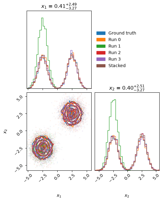
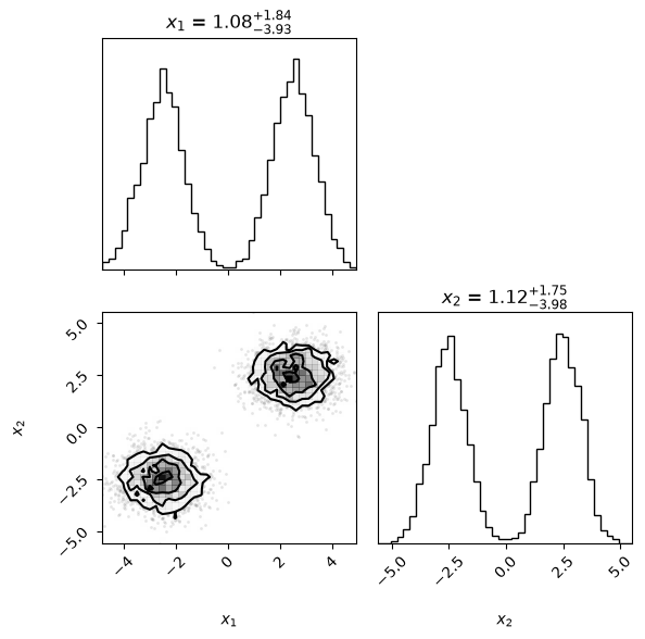
A run that found a single mode places all of its mass there, while the stacked posterior recovers both modes in the right proportions. stacked.plot() draws the corner plot of the stacked posterior alone:

fig = stacked.plot(n_samples=n_samples, figsize=(6, 6), bins=40)

5. Save and load the stacked posterior

stacked.save(file) writes the whole object to a file: the retained posteriors, the optimized weights, the ELBO report and the state of the random generator. SVBMC.load(file) reads it back. As with vp.save, .pkl is added to a name without an extension, and save raises FileExistsError rather than replace an existing file unless overwrite=True. The file holds no Python bytecode, so it can be loaded under another Python version, and loading needs no torch: a loaded stack can be sampled and plotted without it.

stacked.save("stacked_posterior.pkl", overwrite=True)

restored = SVBMC.load("stacked_posterior.pkl")
print("Same weights:      ", np.array_equal(restored.w, stacked.w))
print("Same headline ELBO:", restored.elbo == stacked.elbo)

Same weights:       True
Same headline ELBO: True

6. Conclusions

• Run PyVBMC several times on the same model and data, then pass the returned posteriors to SVBMC and call optimize(); the stacked posterior needs no new model evaluations.

• Read the stacked ELBO estimate from scalar stacked.elbo, which on a noisy target is normally a shrinkage estimate; inspect stacked.elbo_details for the raw, shrinkage, capped and naive estimates, and interpret stacked.elbo_sd as uncertainty of the raw evaluation at the selected weights.

• The runs must describe the same model and data, which the object cannot check; it refuses runs that differ in the number of parameters or in the hard bounds.

• stacked.sample(n, balance_flag=True) stratifies the draws: each run contributes within one draw of its exact share of the weights, and within a run the draws follow the component weights through the balanced allocation of VariationalPosterior.sample (lower variance for expectations, not an independent sample).

• Keep a stack with stacked.save(file) and restore it with SVBMC.load(file).

For details, see the S-VBMC paper: Silvestrin, F., Li, C., & Acerbi, L. (2025). Stacking Variational Bayesian Monte Carlo. Transactions on Machine Learning Research. arXiv:2504.05004. Please cite it together with the VBMC and PyVBMC papers when you use S-VBMC.

Acknowledgments

Work on the PyVBMC package is supported by the Research Council of Finland (grants 356498 and 358980 to Luigi Acerbi) and its Flagship programme: Finnish Center for Artificial Intelligence FCAI.